FCC-ee tutorial using HepSim files
Here is mini-tutorial explaining how to use Monte Carlo truth-level files from the HepSim for the FCC-ee studies. The setup of the computer environment is described in this section. The HepSim part of this tutorial does not require CVMFS and can be done on any computer with java installed.
FCC-ee tutorial
See https://hep-fcc.github.io/fcc-tutorials/ The source files are on GitHub at https://github.com/HEP-FCC/fcc-tutorials. Check this for making contributions: https://hep-fcc.github.io/fcc-tutorials/CONTRIBUTING.html
Using files from HepSim
This part of the tutorial does not use any C++ specific libraries and can be done on any computers with Java installed. Check java:
java -version
Typically, it will tell openjdk version “1.8.0_352” or higher Java version.
bash   #  set bash if you haven't done this before
wget https://atlaswww.hep.anl.gov/hepsim/soft/hs-toolkit.tgz -O - | tar -xz;
source hs-toolkit/setup.sh
Let's look at a few events: Z→ Z H, where Z→ nunu, and H decays to bbar. The CM energy is 250 GeV. The sample is described in https://atlaswww.hep.anl.gov/hepsim/info.php?item=353
First, print all files with Higgs processes:
hs-find higgs
Then grab the file with H to bbar at e+e-:
hs-ls gev250ee_pythia8_zhiggs_nunubbar
Let's download 10 files (in 2 threads):
hs-get gev250ee_pythia8_zhiggs_nunubbar data 2 10
We should have 10 files in the directory “data”. Let's take a look at a single file. We what to check how many events in the file, how many events etc:
hs-info data/gev250ee_zh_nunubb_001.promc
Do you want to print 1st event? Do this:
hs-info data/gev250ee_zh_nunubb_001.promc 1
Want to examine the log file? Do this:
hs-log data/gev250ee_zh_nunubb_001.promc
Let's study each event in the GUI mode (needs X-session!). Start this GUI and click each event number using the left panel.
hs-view data/gev250ee_zh_nunubb_001.promc
Validation
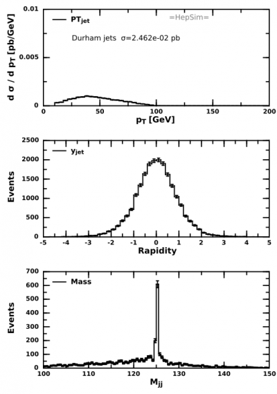
Now we know a lot about this files. Let's make a simple code to run over 10,000 events (2 files) and draw some useful histograms. Click the tab below to see the code. This code may look rather long, but it does a lot: It reads the truth-level events, reconstructs jets, and makes plots of the pT (differential cross section), Rapidity distribution and the invariant mass of the 2 jets. It also saves the image in SVG file and an XML file for examination:
Copy the code shown below to a file “validatation.py” and run it as
hs-run validatation.py
It will create the image with jets and a Higgs peak for 2-jet mass.
Data streaming
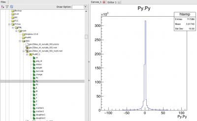
One can also analyze truth-level files using data streaming, i.e. without downloading the actual input files. This example shows data for Higgs to bbar at 240 GeV e+e-. Click the code shown below, save it as “example.py” and run it inside Jas4pp (https://atlaswww.hep.anl.gov/asc/jas4pp/) or using hs-tools package (as “hs-run example.py”).
If you run this code as Jython script inside Jas4pp, you will see a histogram updated in real time:

Analysis of LCIO files
Full example of how to analyse LCIO files is given in: https://atlaswww.hep.anl.gov/asc/wikidoc/doku.php?id=asc:jas4pp#reading_lcio_files
Preparation for fast simulation
For fast simulations we need to install the C++ ProMC library. After it is installed, the compiled Delphes program can start using the ProMC files natively. Let's take this package from https://atlaswww.hep.anl.gov/asc/promc/ and install it. Make sure you have the gcc compiler , zip library (run “yum install python-pip python-setuptools zlib1g-dev zlib-devel” if you do not have them) and CERN ROOT. If you are using CERN or OSG login nodes, you can get these packages as:
Use the key4hep setup with gcc11. It will also link the ROOT libraries:
source /cvmfs/sw.hsf.org/key4hep/setup.sh
If ( /cvmfs/sw.hsf.org/key4hep/ ) is not available on your system, use the older gcc8 version:
source /cvmfs/sft.cern.ch/lcg/views/LCG_97/x86_64-centos7-gcc8-opt/setup.sh
Then install ProMC (currently it is an external package):
wget http://atlaswww.hep.anl.gov/asc/promc/download/current.php -O ProMC.tgz
tar -zvxf ProMC.tgz
cd ProMC
./build.sh                      # build all source files
./install.sh lib               # install into the "lib" directory
source lib/promc/setup.sh  # make it available
After the installation, make sure you see a bunch of executable files:
echo $PROMC/bin
This package will be used for fast simulation. In addition, you can perform various transformation of the event records. For example, move your data to ROOT:
cd $PROMC/examples/promc2root
make                          # creates converter promc2root
cd ../../../../../data/   # navigate to the directory with data
$PROMC/examples/promc2root/promc2root gev250ee_zh_nunubb_001.promc  gev250ee_zh_nunubb_001_truth.root
Note some system picks the native “zlib library”. If you see an error in compilation, remove “-lz” string on the line 23 of Makefile.
The last command will create ROOT files with the tree “ProMC”:
Similarly, one can do transformation oto the popular text formats: See
$PROMC/examples/promc2lhef
$PROMC/examples/promc2hepmc
The same directory “examples” contains the reverse transformations.
Creating Pythia8 events
In this example, instead of downloading files with e+e- events, we will generate Pythia8 events at the truth level. We create 100k events at 250 GeV CM energy with all Higgs processes. Then we will force H to decay to 2 b jets.
(1) Step 1. Get the package:
wget https://atlaswww.hep.anl.gov/hepsim/examples/package_ee.tgz
tar -zvxf package_ee.tgz
(2) Compile the program. The steering card is located in “cards” that defines how many events and what are the processes.
cd package_ee
make
(3) Run the Pythioa8 events using the supplied bash script. This creates 10 output files in the directory “out”. You can view the output and the log file as
./A_RUN_gev250_higgs_bbar
This script creates the output file in the directory “out”. One can view events in this file as:
cd out
promc_browser gev250ee_higgs_bbar_001.promc
Fast simulation
To perform fast simulation, install Delphes using the standard steps:
wget http://cp3.irmp.ucl.ac.be/downloads/Delphes-3.5.0.tar.gz
tar -zxf Delphes-3.5.0.tar.gz
cd Delphes-3.5.0
make
On some systems, the compilation may fail if the ZLIB library is already present, i.e. the error will be “inflateValidate@ZLIB”. In this case, remove “-lz” on the line 45 of the Makefile.
The last line of the compilation should have “DelphesProMC” (binary file to process events).
cd ..
./Delphes-3.5.0/DelphesProMC  ./Delphes-3.5.0/cards/delphes_card_CircularEE.tcl \
data/gev250ee_zh_nunubb_001.root  \
data/gev250ee_zh_nunubb_001.promc
The output file will be data/gev250ee_zh_nunubb_001.root
Full simulation and file conversions
For full simulations, we will need to convert ProMC files to the LCIO files. You can use the converter posted to https://github.com/hepsim-org/promc2other Read the README of this simple tool.
The C++ version of the ProMC package can also convert files to HEPMC2 and LHEF. Look at the directories:
cd $PROMC/promc2hepmc   # tool to convert to HEPMC2
cd $PROMC/promc2lhe         #  tool to convert to LHEf
The key4hep requires HEPMC3 format (not HEPMC2). Therefore, the current option is to convert PROMC to HEMC2 and then convert HEPMC3. Alternatively, key4hep can take LHE files.
First, get the script:
wget http://fccsw.web.cern.ch/utils/converters/lhe2edm.sh
Then use it like this:
$ source /cvmfs/sw.hsf.org/key4hep/setup.sh
$ ./lhe2edm.sh inputfile.lhe output.edm [--nevt=1000] [--stable]
You can specify the number of events in the file in the case the guess based on grepping <event> is wrong.
If you specify ‘—stable’ only the stable particles (status == 1) are kept in the final file.
Some outreach
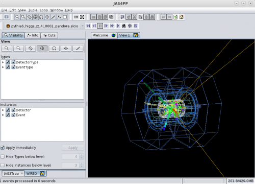
If you are a student who has never seen a typical e+e- event in real life, you may use this simple tool to display and view e+e- events. Here we will explore typical e+e- events at the CM energy 250 GeV with Higgs decaying to two Z bosons. Then Z-bosons decay to 4 leptons. The events will be visualized in the SID detector from the ILC project (events for FCC-ee will not look very different, but the FCC-ee detector will have somewhat different geometry). The program uses Jas3/Wired display used for the ILC R&D.
Unlike the tutorial discussed above, this example only requires a personal Linux/Windows/Mac computer with Java installed. It will use the Jas4pp program and files from HepSim.
wget https://atlaswww.hep.anl.gov/asc/jas4pp/download/jas4pp-1.7.tgz
tar -zvxf jas4pp-1.7.tgz
cd jas4pp
wget https://mc.hep.anl.gov/asc/hepsim/events/ee/250gev/pythia6_higgs_zz_4l/rfull001/pythia6_higgs_zz_4l_0001_pandora.slcio
jaspp pythia6_higgs_zz_4l_0001_pandora.slcio
You will see an editor. Use the left panel and expand “DataSets”. Then go to “File→New→Wired 4 View. You will see a black screen. The press the small blue arrow from the top menu. It is called “Go”.
You can also display very busy events with H→ bbar if you will download files from 151rfull001 link.
You can explore various detector components, data collections etc. Use File→New→LCSim event browse. etc. You can also display other collision processes and different detectors using the HepSim repo.
— Sergei Chekanov 2023/04/03 21:08