Table of Contents
Plotting distributions
HepSim repository can be used to reconstruct any distribution or differential cross section using truth-level files. Many HepSim MC samples include *.py scripts to calculate differential cross sections. You can run them using downloaded ProMC files (in which case you pass the directory with *promc files as an argument). The second approach is to run *.py scripts on a local computer without downloading ProMC files beforehand. In this case, data will be streamed to computer's memory and processed using your algorithm.
You can create plots using a number of programming languages, Java, Python, C++, Ruby, Groovy etc. Plots can be done on any platform, without modifying your system. C++ analysis programs require ROOT and Linux.
Below we will discuss how to analyse HepSim data using Java, since this approach works on any platform (Linux, Mac, Windows) and does not require installation of any platform-specific program. As before, make sure that Java 7 and above is installed (check it as “java -version”).
Method I. Running in a batch mode without downloaded ProMC files
You can run validation scripts in a batch mode as:
wget http://mc.hep.anl.gov/asc/hepsim/events/pp/100tev/ttbar_mg5/macros/ttbar_mg5.py
hs-run ttbar_mg5.py
Another approach is to use Jas4pp or DataMelt. Such programs give more flexibility and more libraries for analysis. In this example, we will run a Python script that downloads data from URL into the computer memory and runs it in a batch mode. First, you will need an analysis code from HepSim. Look at ttbar sample from Madgraph: ttbar_mg5. Find the URL location of the analysis script (“ttbar_mg5.py”) located at the bottom of this page. Then copy the URL link of the file *.py using the right mouse button (“Copy URL Location”). Let us make a calculation of differential ttbar cross section.
Here is how to process the analysis using Jas4pp:
wget http://atlaswww.hep.anl.gov/asc/jas4pp/download/current.php -O jas4pp.tgz
tar -zvxf jas4pp.tgz
cd jas4pp
source ./setup.sh # takes 5 sec for first-time optimization
wget http://mc.hep.anl.gov/asc/hepsim/events/pp/100tev/ttbar_mg5/macros/ttbar_mg5.py # get the HepSim script
fpad ttbar_mg5.py # process it in a batch mode.
Look at the “example” directory of the Jas4pp installation. It has a several examples of how to process the ProMC files.
Similarly, you can use a more complex DataMelt:
wget -O dmelt.zip http://jwork.org/dmelt/download/current.php                        # get DataMelt
wget http://mc.hep.anl.gov/asc/hepsim/events/pp/100tev/ttbar_mg5/macros/ttbar_mg5.py #  analysis script
unzip dmelt.zip
./dmelt/dmelt_batch.sh ttbar_mg5.py
(first time it will run slower since it needs to rescan jar files). In this example, data with the URL (given inside ttbar_mg5.py) will be downloaded to the computer memory. You can also pass URL with data as an argument and limit the calculation to 10000 events:
./dmelt/dmelt_batch.sh ttbar_mg5.py http://mc.hep.anl.gov/asc/hepsim/events/pp/100tev/ttbar_mg5/ 10000
If you want to see a pop-up canvas with the output histogram on your screen, change the line “c1.visible(False)” to “c1.visible()” and comment out “sys.exit(0)” at the very end of the “ttbar_mg5.py” macro. You can change the output format from “SVG” to “PDF”, “EPS” or “PNG”. Look at the Java API.
Method II. Running in a batch mode after downloading ProMC files
The above approach depends on network availability at the time when you do the analysis. It is more convenient to download data files first and run over the data. If all your ProMC files are in the directory “data”, run this example code from the DataMelt directory:
./dmelt/dmelt_batch.sh ttbar_mg5.py data
Here is a complete example: we download data to the directory “ttbar_mg5”, then we download the analysis script, and then we run this script over the local data using 10000 events:
wget http://mc.hep.anl.gov/asc/hepsim/events/pp/100tev/ttbar_mg5/macros/ttbar_mg5.py # get analysis scrip
hs-get http://mc.hep.anl.gov/asc/hepsim/events/pp/100tev/ttbar_mg5 ttbar_mg5
./dmelt/dmelt_batch.sh ttbar_mg5.py ttbar_mg5 10000
Similarly, you can use Jas4pp.
Method III. Running in a GUI mode
You can perform short validation analysis using an editor as:
hs-ide ttbar_mg5.py
Run this code by pressing “run”. This approach uses a light-weight editor built-in inside the hs-tool package.
For Jas4pp, you can start an editor, correct the script, and run it:
./jaspp ttbar_mg5.py # Open the script in the editor
Then, use the right mouse button and select “Run Python”. You will see the output.
For the DMelt IDE, you can also bring up a full-featured GUI editor as this:
./dmelt/dmelt.sh ttbar_mg5.py
It will open the Python script for editing. Next, run this script by clicking the image of green running man on the status bar (or press [F8]).
Method IV. Running in a GUI mode using URL dialog
If you use DMelt, you can run this code using a more conventional editor:
../dmelt/dmelt.sh
On Windows, click “dmelt.bat”. Then find a HepSim analysis script with the extension *.py. You can do this by clicking “Info” column in the HepSim database. For example, look at the ttbar sample from Madgraph ttbar_mg5. Find the URL location of the analysis script with the extension *.py located in the bottom of this page. Then copy the URL link of the file *.py using the right mouse button (“Copy URL Location”). Next, in the DataMelt menu, go to [File]→[Read script from URL]. Copy the URL link of the *.py file to the pop-up DataMelt URL dialog and click “run” (or [F8] key). The program will start running with the output going to “Jython Shell”. When processing is done, you will see a pop-up window with the distribution.
If you have already analysis file, you can load it to the editor as:
./dmelt/dmelt.sh ttbar_mg5.py
and run it using “run” or [F8] key.
Event view in 3D
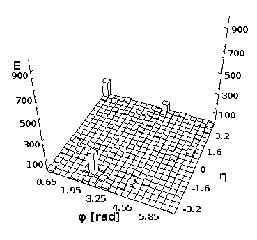
You can look at separate event and create a 2D lego plot for separate events using Python and Java. First, download any ProMC file, i.e.
wget http://mc.hep.anl.gov/asc/hepsim/events/pp/100tev/qcd_pythia8/pythia100qcd_001.promc
Then, execute this script in DatMelt which fills 2D histogram with final-state particles:
The execution of this script will bring-up a window with the lego plot.
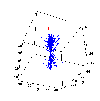
You can also look at a simple “tracking” for a given event:
The code written in Python is attached:
Reading NLO predictions
NLO records are different from showered MC. There is much less information available on particles, and events have weights. In many cases, PDF uncertainties are included. Here is an example how to read outputs from the MCFM program generated on BlueGene/Q at ANL.
hs-view http://mc.hep.anl.gov/asc/hepsim/events/pp/100tev/gamma_mcfm/gamma100tev_0000000.promc
or:
wget http://mc.hep.anl.gov/asc/hepsim/events/pp/100tev/gamma_mcfm/gamma100tev_0000000.promc
hs-view gamma100tev_0000000.promc
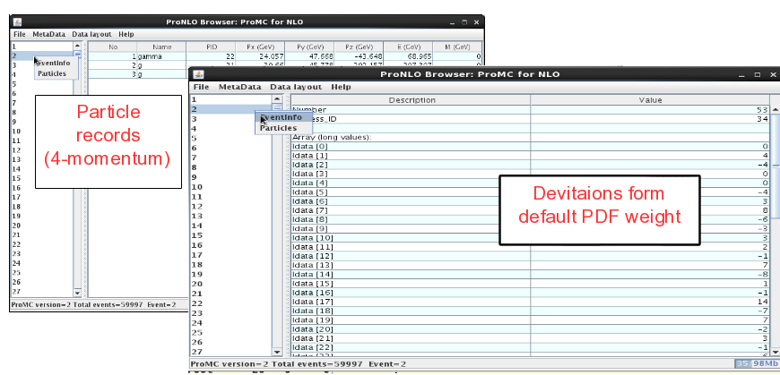
On the left panel, click on the event and then look at “Event info”. It shows the integer values (idata) that encode the PDF uncertainties, while the float array (“fdata”) shows other information. The first element in the float array is the weight of the event. The particle information is shown as usual (but without mother ID etc.).
The scripts that reconstruct cross sections are attached to the HepSim event repository. Here is how to run a script to reconstruct a direct-photon cross section at NLO QCD using DatMelt:
You can also open a script as:
wget http://mc.hep.anl.gov/asc/hepsim/events/pp/8tev/gamma_jetphox.py
./dmelt.sh gamma_jetphox.py
Alternatively, open this script in the DMelt editor and press run (or [F8]).
NLO event record includes 4-momenta of particles and event weights (double values). In addition, deviations form central weights are included as an array of integer values as:
You can calculate differential cross sections using online files using this example:
mkdir Higgs; cd Higgs;
wget http://mc.hep.anl.gov/asc/hepsim/events/pp/100tev/higgsjet_gamgam_mcfm/macros/higgsjet_gamgam_mcfm.py
wget -O dmelt.zip http://sourceforge.net/projects/dmelt/files/latest/download
unzip dmelt.zip
./dmelt/dmelt_batch.sh higgsjet_gamgam_mcfm.py http://mc.hep.anl.gov/asc/hepsim/events/pp/100tev/higgsjet_gamgam_mcfm/
This example runs “higgsjet_gamgam_mcfm.py” code using online files and creates a Higgs differential cross section with PDF uncertainties. We use DMelt to do the calculations (after updating one jar file). You can also use ROOT/C++ to do the same.
Using C++/ROOT
To read downloaded ProMC files using C++/ROOT, you need to install the ProMC and ROOT package. If not sure, check these environmental variables:
echo $ROOTSYS
echo $PROMC
They should point to the installation paths. If you use CERN's lxplus or AFS, simply one can setup PROMC as:
source /afs/cern.ch/atlas/offline/external/promc/setup.sh
which is built for x86_64-slc6-gcc48-opt.
Then, look at examples:
  $PROMC/examples/reader_mc/  - shows how read a ProMC file from a typical Monte Carlo generator
  $PROMC/examples/reader_nlo/ - shows how read a ProMC file with NLO calculations (i.e. MCFM)
  $PROMC/examples/promc2root/ - shows how to read PROMC files and create ROOT Tree.
The same example directory shows how to write ProMC writes and convert to other formats.
You can generate an analysis code in C++, Java and CPython from a ProMC file with unknown data layout. Here is an example for a NLO file:
wget http://mc.hep.anl.gov/asc/hepsim/events/pp/8tev/gamma_jetphox/ggd_mu1_45_2000_run0_atlas50.promc
promc_proto ggd_mu1_45_2000_run0_atlas50.promc
promc_code
make
This creates directories with the C++/CPython/Java analysis codes. For a longer description, read the ProMC manual.
For C++/ROOT, you can use this C++/ROOT example package. Untar it and compile using “make”. This will produce “promc2root” executable. It reads all ProMC files in a given directory and fills ROOT histograms with cross sections.
Use this Doxygen description to work with C++:
- annotated classes - for complete MC event records
- annotated classes - for NLO event records
Please look at HepSim programming tutorials on how to design Jython scripts. Please refer ProMC web page on how to read/write ProMC files.
Also, there is a simple example showing how to read Monte Carlo files from HepSim in a loop, build anti-KT jets using FastJet, and fill ROOT histograms. Download hepsim-cpp package and compile it:
    wget http://atlaswww.hep.anl.gov/asc/hepsim/soft/hepsim-cpp.tgz -O - | tar -xz;
    cd hepsim-cpp/;
    make
Read “README” inside this directory. Do not forget to populate the directory “data” with MC files before running this example.
Conversion to ROOT files
The ProMC files can be converted to ROOT files using “promc2root” converter located in the $PROMC/examples/promc2root directory. ROOT files will be about 30-50% larger (and their processing takes more CPU time). Please refer the ProMC manual.
cp -rf $PROMC/examples/promc2root .
cd promc2root
make
./promc2root [promc file] output.root
Converting to LCIO
ProMC files can be converted to LCIO files for full detector simulations. This is an example of such conversion (it requires Java installed):
wget http://atlaswww.hep.anl.gov/asc/promc/download/current.php -O ProMC.tgz
tar -zvxf ProMC.tgz
cd examples/promc2lcio
source setup.sh
javac promc2lcio.java
java promc2lcio file.promc file.slcio
The last commends creates file.slcio with “MCparticle” container.
Converting to other formats
Look at other directories in “examples/”. You can convert ProMC files to many other formats (most converters require installation of the ProMC C++ package).
Extracting events
A file can be reduced in size by extracting N events as this:
hs-extract signal.promc N
where signal.promc is the original file, and N is the number of events to extract.
Comparing MC and data
HepSim maintains analysis scripts that can be used for comparing Monte Carlo simulations with data from Durham HepData database. For example, click the link with AAD 2013 (Search for new phenomena in photon+jet events collected in proton–proton collisions at sqrt(s) = 8 TeV with the ATLAS detector) paper
- Navigate to “DataMelt” and use right-mouse and select “Copy link location”
- Start DMelt if you did not yet, and select [File]-[Read script from URL]. Copy and paster the URL link from the HepData database
- Click “run”.
HepData maintain Jython scripts that use the same syntax as HepSim. You can start from a HepSim validation script, and before the “export” command, append the scripts with data from Durham HepData database. Or you can start from a HepData “SCaVis” script and add parts from HepSim validation script that reads data from HepSim. Note that SCaVis and DMelt are equivalent.
XML output format
Many scripts of HepSim create SVG images and a cross platform JDAT data format based on HBook. In order to convert JDAT files into CPython or ROOT object, read the data using xml.dom. This is a conversion to the CPython:
Programming with HepSim
Please look at the tutorials which show how to create Python/Jython scripts to read ProMC files.
Send comments to: — Sergei Chekanov (ANL) 2016/02/08 10:26


