Table of Contents
Jet mass for CA12
This page discusses CA12 only. For antiKT6 and antiKT10, see the last section of this wiki.
Detector-level distributions
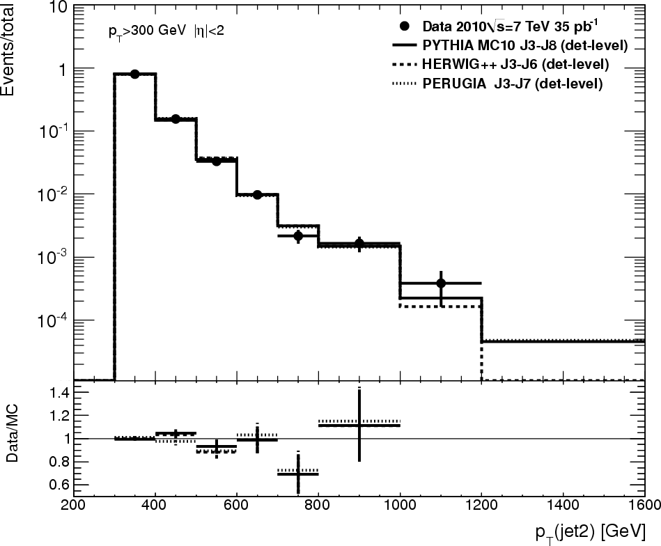
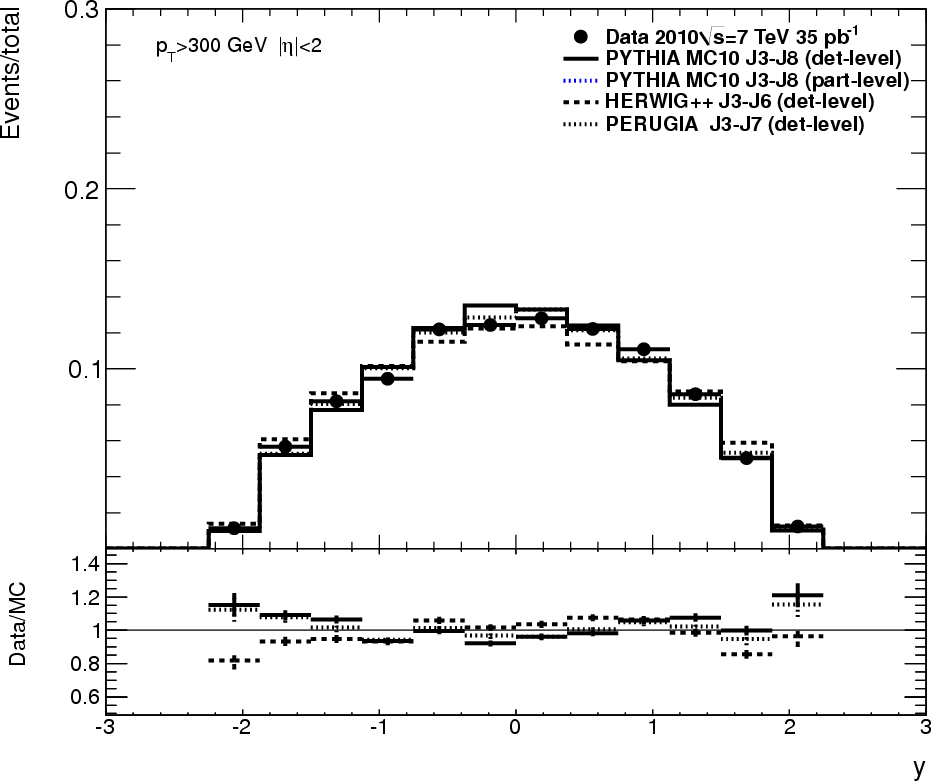
Detector level pT and Eta. Default cuts. Single-vertex cut is used for central values.
- det_jet1_Pt.eps.png - Lead pT jet, det_jet2_Pt.eps.png - 2nd pT jet
- det_jet1_Eta.eps.png - Eta for all jets above pT>300 GeV
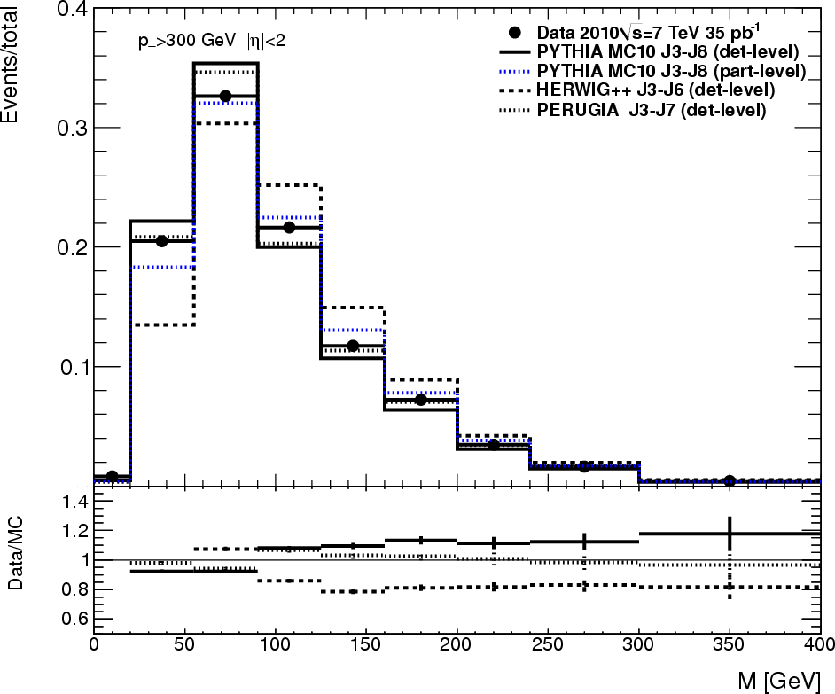
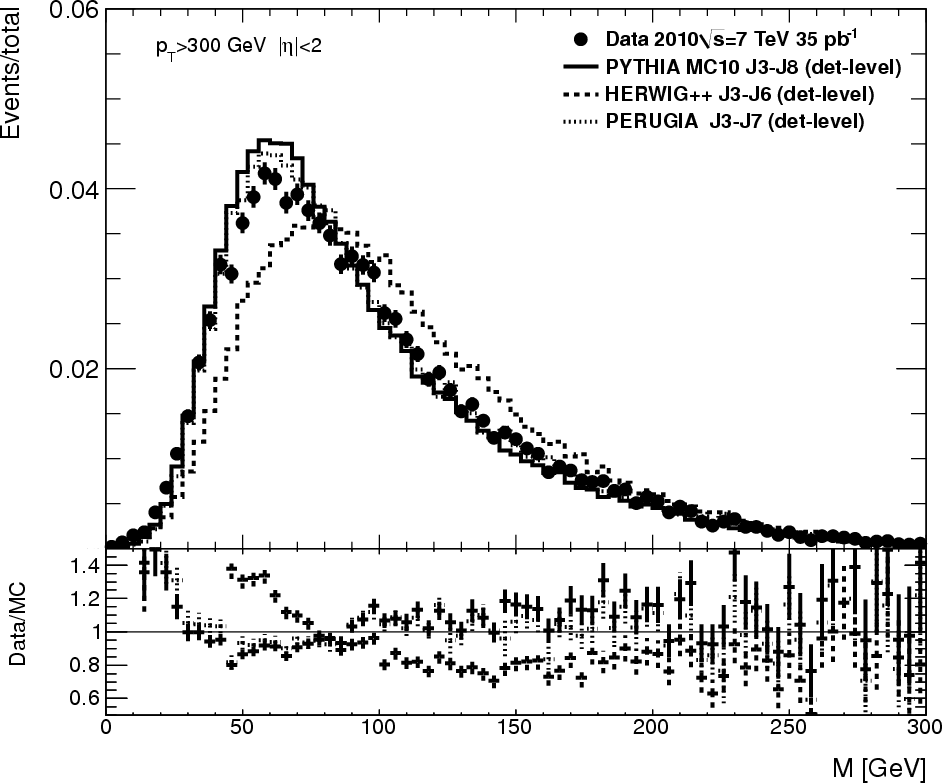
Jet masses at the detector level:
- det_jets_m.eps.png - All jets for wide bins
- det_jets_m.eps.png - All jets for small bins
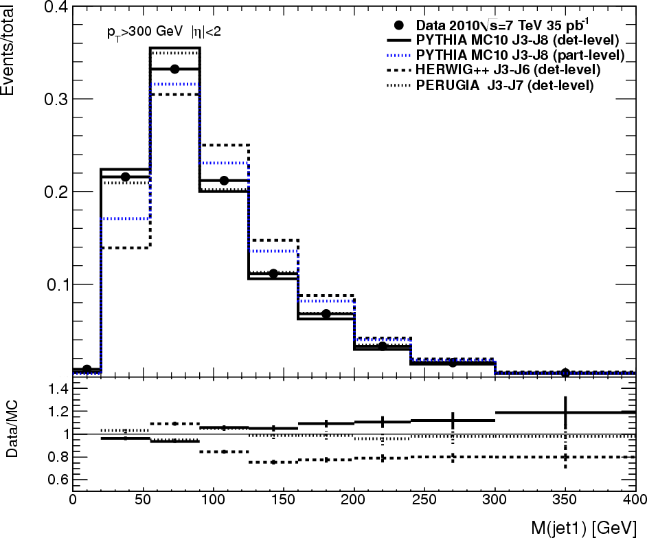
- det_jet1_m.eps.png - 1st jet for wide bins
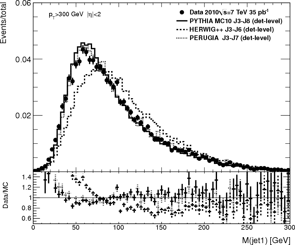
- det_jet1_ms.eps.png - 1st jet small bins
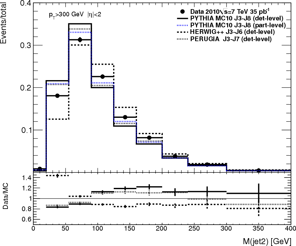
- det_jet2_m.eps.png - 2nd jet for wide bins,
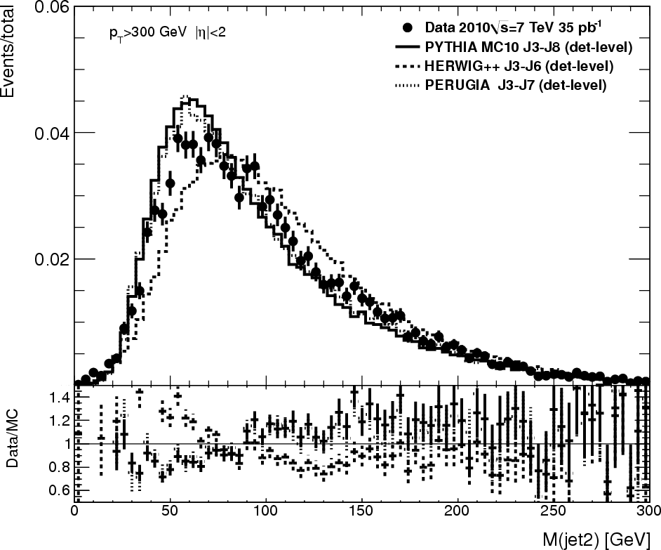
- det_jet2_ms.eps.png - 2nd jet small bins
(to get EPS, remove “png” extension)
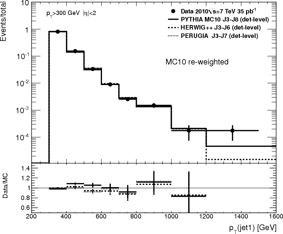
Detector level pT and Eta. MC10 reweighted in mass for unfolding (systematics 1). Only leading in pT jets are shown
- det_jet1_Pt.eps.png - pT
- det_jet1_m.eps.png - wide bins
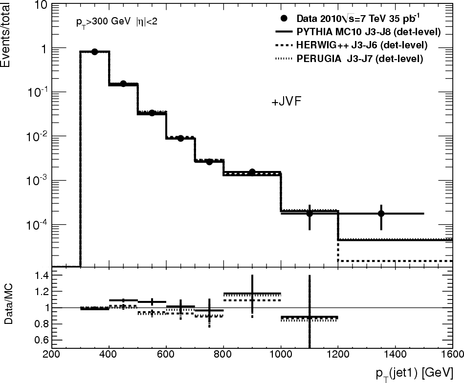
Detector level pT and Eta. Additional JVF cut for systematics (systematics 3). Only leading in pT jets are shown
- det_jet1_Pt.eps.png - pT
- det_jet1_m.eps.png - wide bins
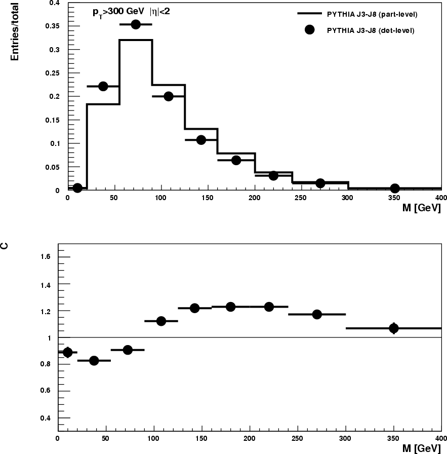
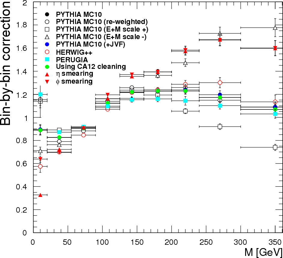
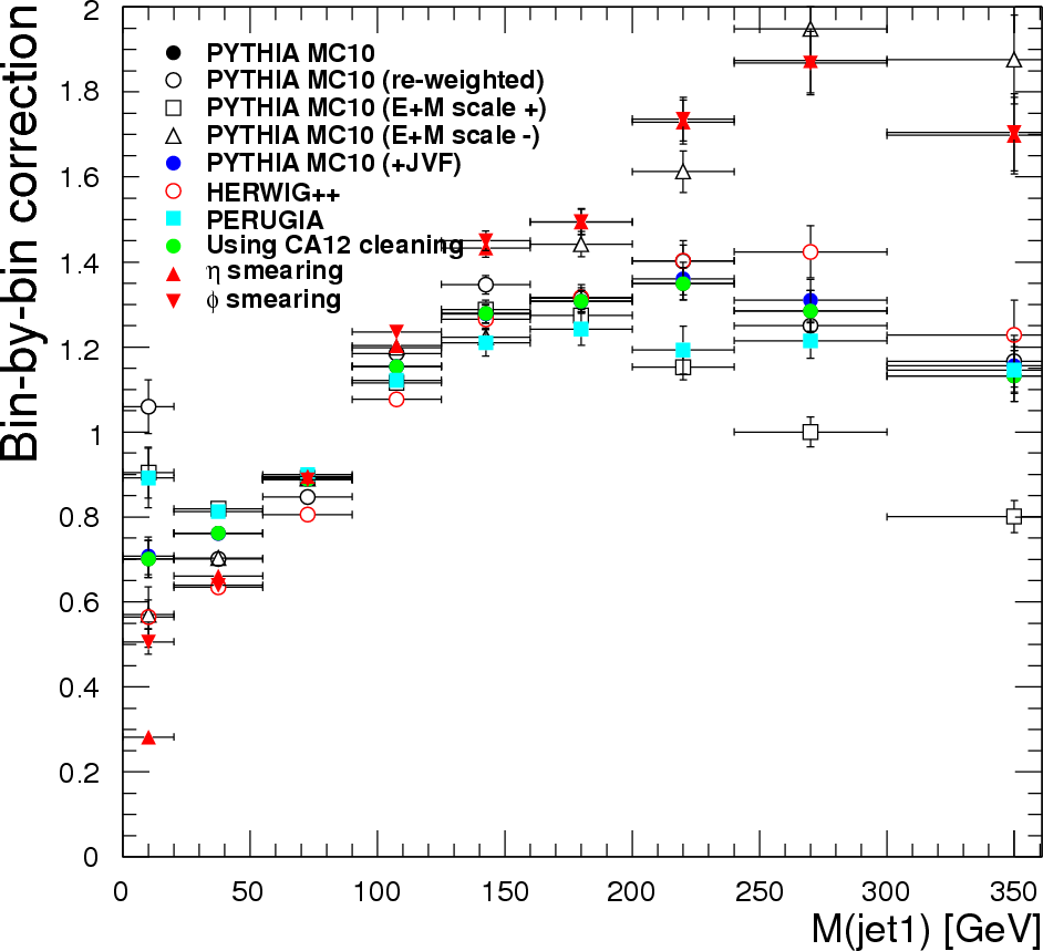
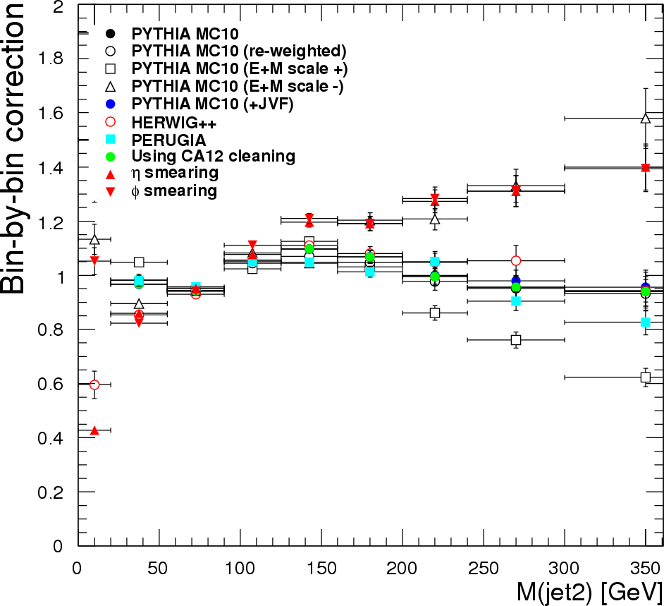
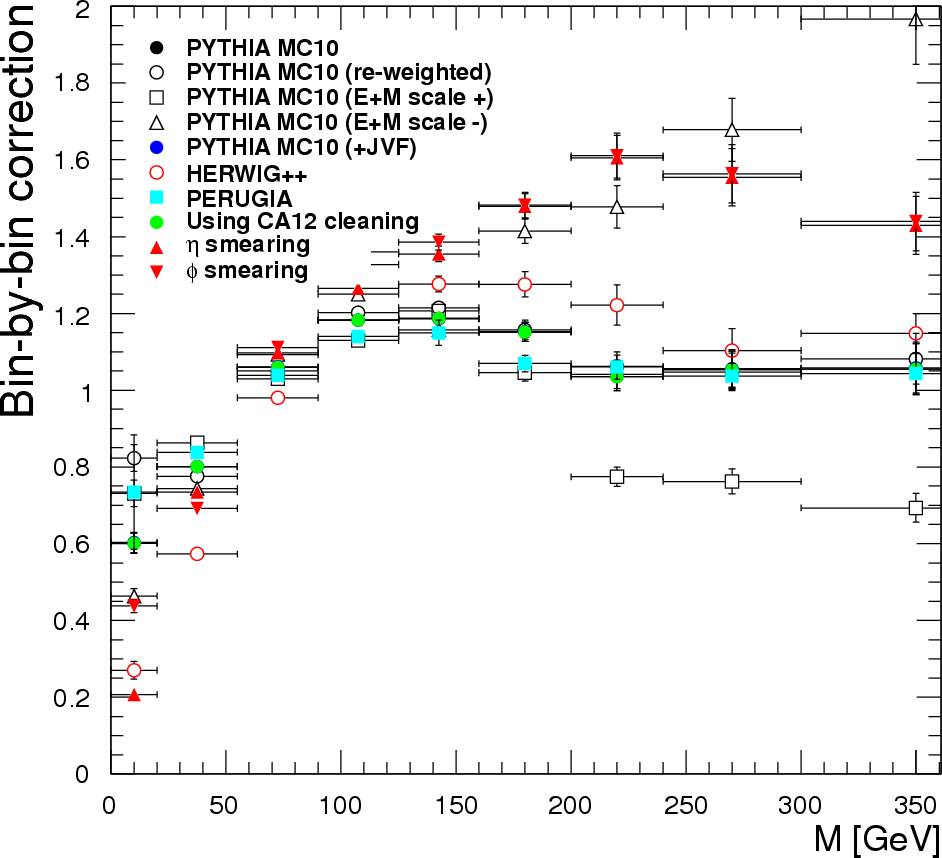
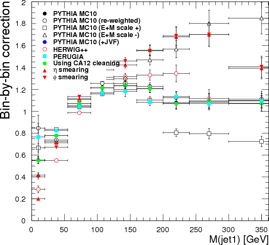
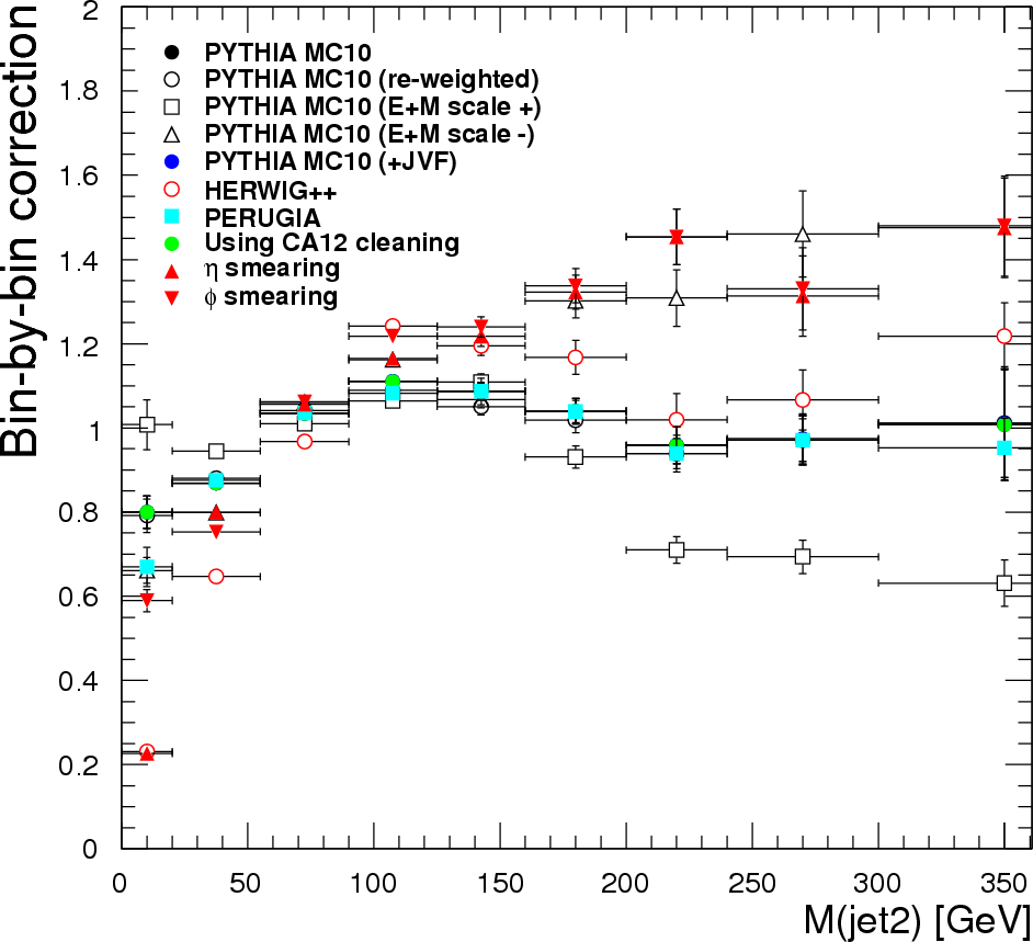
Bin-by-bin correction factors
- corr_Jets_mass.eps.png - All jets for PYTHIA MC10
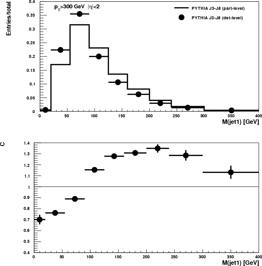
- corr_Jet1_mass.eps.png - 1st jet for PYTHIA MC10
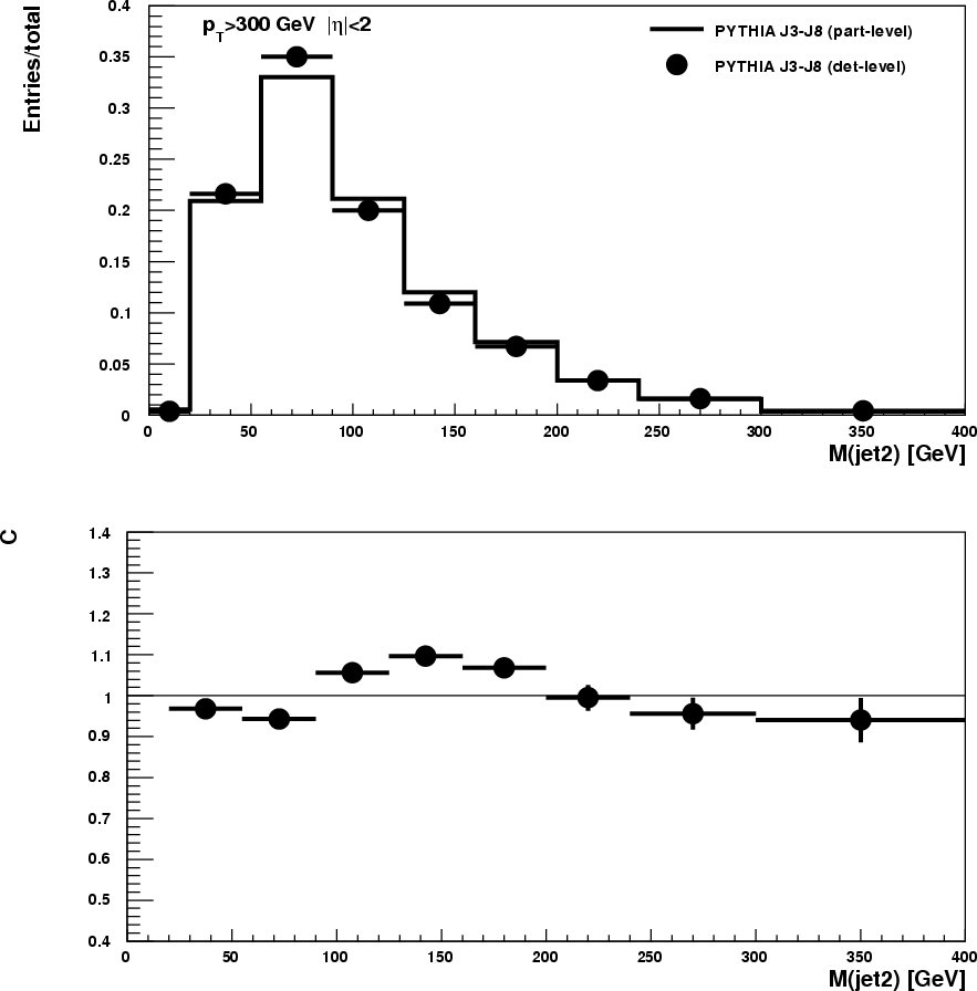
- corr_Jet2_mass.eps.png - 2nd jet for PYTHIA MC10
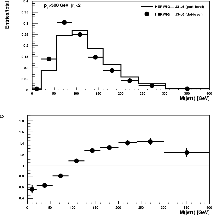
- corr_Jet1_mass_hrw.eps.png - 1st jet for HERWIG++
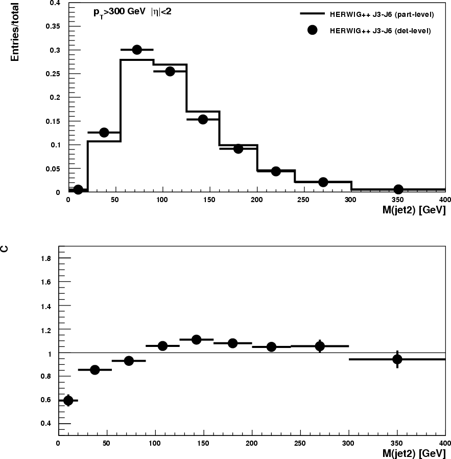
- corr_Jet2_mass_hrw.eps.png - 2nd jet for HERWIG++
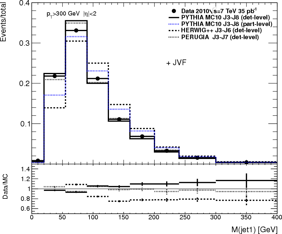
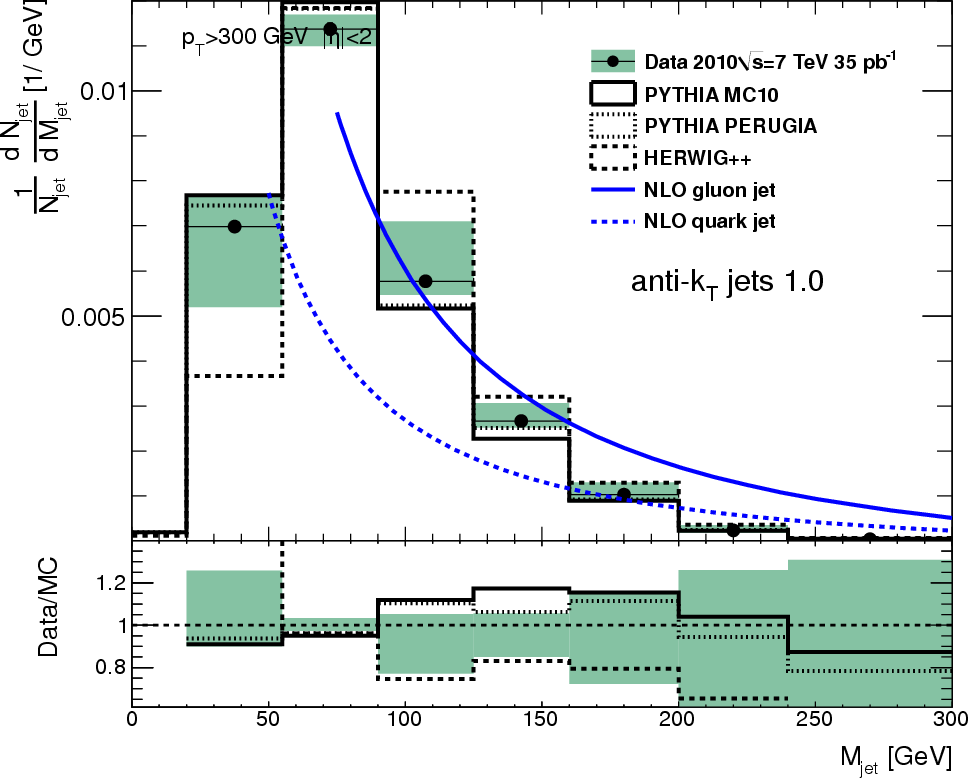
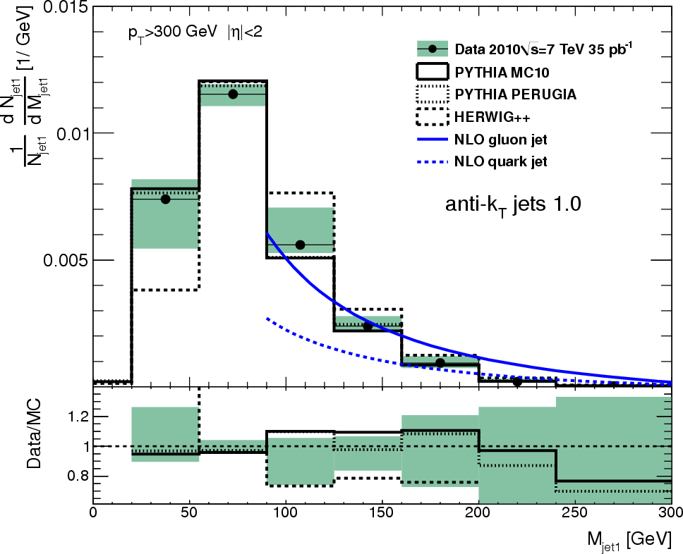
Final results for CA12
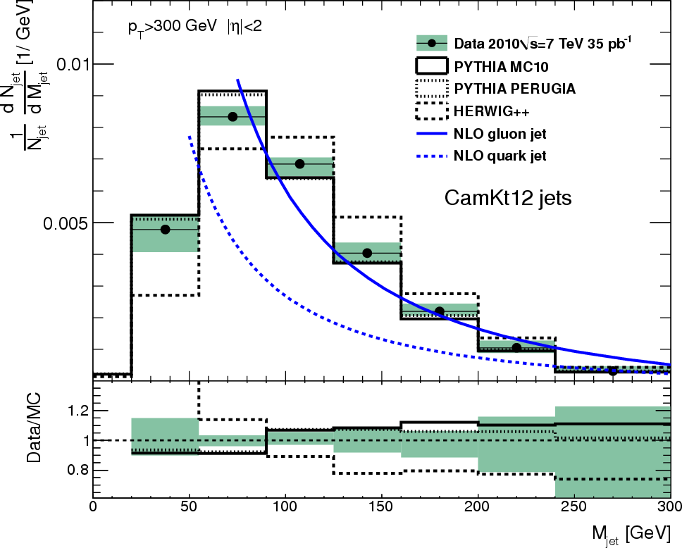
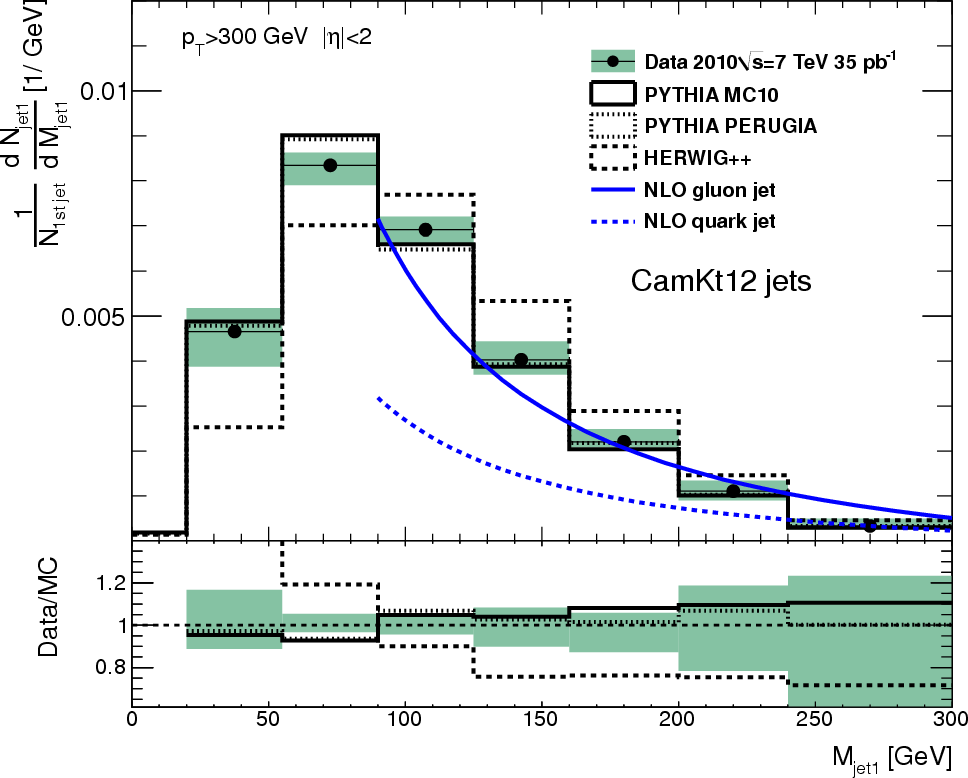
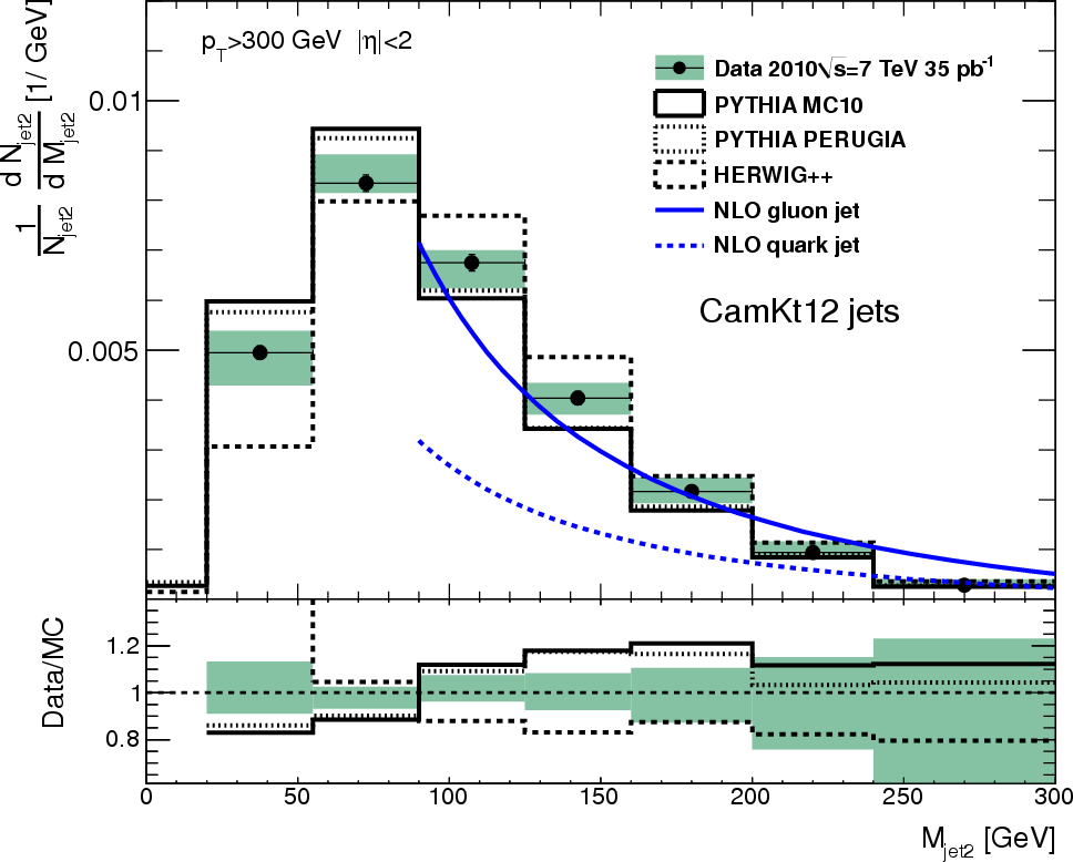
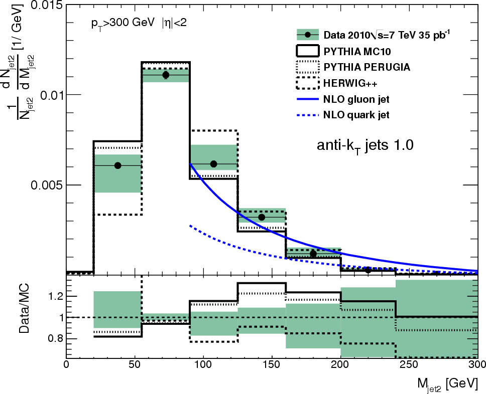
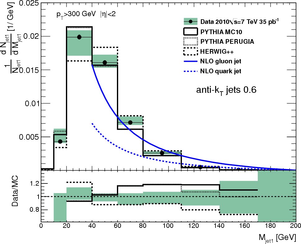
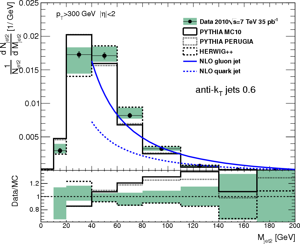
Particle-level results compared to the truth-level MC generators. First bin is removed in the data.
- final_jets_m.eps.png - All jets
- final_jet1_m.eps.png - 1st lead jet
- final_jet2_m.eps.png - 2nd lead jet
In addition, results using smaller (“discovery”) bins without detector unfolding:
- det_jets_m.eps.png - All jets
- det_jets_m.eps.png - 1st lead jet
- det_jets_m.eps.png - 2nd lead jet
Systematical uncertainties
- Central values using the default cuts
- Re-weighted PYTHIA MC10 to describe the data
- Energy scale and mass scale uncertanty. Jet pT and E was scaled by +/-4, while the mass was scaled by +/- (4 + X)% where X is determined from Fig.2 of the not (right), and changes as 4% (M<50 GeV), 1% (50<M<150 GeV) and 5% (150<M<250 GeV) and 5% (M>250 GeV)
- JVF=1 in addition to the single vertex cut
- HERWIG++ to recalculate bin-by-bin corrections (dependence on fragmentation)
- PYTHIA Perugia tune to recalculate bin-by-bin corrections (dependence on UE modeling)
- Removing the antiKT6 cleaning cut for fat jets (CA12 and antiKT10)
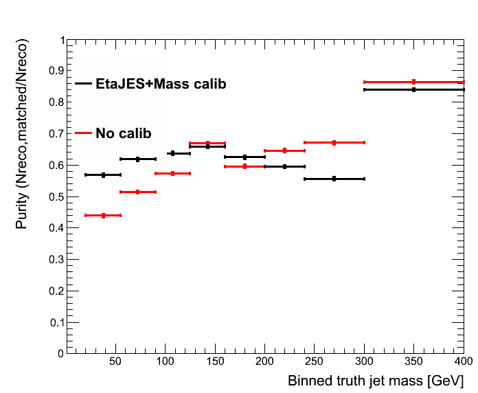
In addition, alternative calibration (only E, pT and Eta. No mass calibration) was checked (both MC and data are affected).
Bin-by-bin correction factors for 5 systematics checks:
- corr_jets_m.eps.png - all jets (leading and subleading)
- corr_jet1_m.eps.png - 1st lead. jet
- corr_jet2_m.eps.png - 2nd lead jet
Table with % contributions: sys_ratio.csv lists systematical uncertanties of each cut variation in % to the total mass value
Tables with the central values for bin-by-bin unfolding with the systematical uncertainties (added in quadrature). The unsertanties are symmetrized.
- Jets_mass_correction.txt - all jets (leading and subleading)
- Jet1_mass_correction.txt - 1st lead. jet
- Jet2_mass_correction.txt - 2nd lead jet
Jetphox prediction
Jetphox predictionals are based on Jetphox1.3 generating ROOT ntuples using the same bins in pT as for the final plots.
Theoretical predictions and publications
http://arxiv.org/abs/0810.0934
http://www-cdf.fnal.gov/physics/new/qcd/BoostedJets/public_note.pdf
http://arxiv.org/abs/1001.5027
CDF analysis http://www-cdf.fnal.gov/physics/new/qcd/BoostedJets/index.html
http://arxiv.org/abs/1104.1646 Jet substructure
Final results for antiKT10
Particle-level results compared to the truth-level MC generators. First bin is removed in the data.
- final_jets_m.eps.png - All jets
- final_jet1_m.eps.png - 1st lead jet
- final_jet2_m.eps.png - 2nd lead jet
Bin-by-bin correction factors for the 5 systematics checks:
- corr_jets_m.eps.png - all jets (leading and subleading)
- corr_jet1_m.eps.png - 1st lead. jet
- corr_jet2_m.eps.png - 2nd lead jet
Table with % contributions: sys_ratio.csv lists systematical uncertanties of each cut variation in % to the total mass value
Tables with the central values for bin-by-bin unfolding with the systematical uncertainties (added in quadrature). The unsertanties are symmetrized:
- Jets_mass_correction.txt - all jets (leading and subleading)
- Jet1_mass_correction.txt - 1st lead. jet
- Jet2_mass_correction.txt - 2nd lead jet
AntiKT10 jet figures: www link
Final results for antiKT6
Particle-level results compared to the truth-level MC generators. First bin is removed in the data.
- final_jet1_m.eps.png - 1st lead jet
- final_jet2_m.eps.png - 2nd lead jet
Other plots with correction factors, detector-level distributions for antiKT10 and antiKT6 jets are given below:
AntiKT6 jet: www link
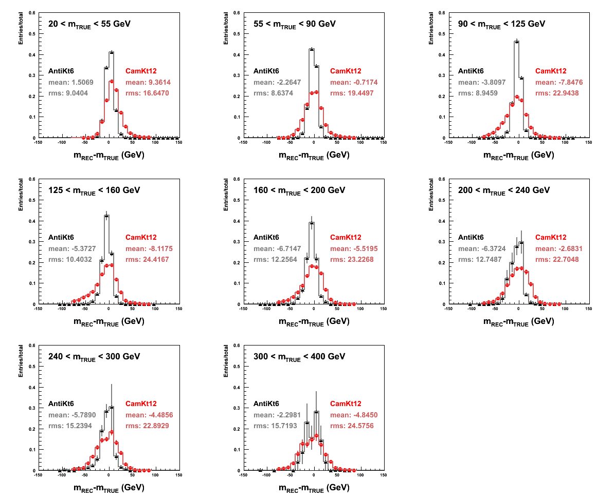
Calibration: mass resolution and efficiency/purity
The absolute mass resolution for AntiKt6LCTopo and CamKt12LCTopo jets (Mass of reco jet minus mass of truth-matched truth jet) is plotted in truth mass bins for the leading jet in each event passing selection cuts (jet1pT>300GeV, jet1|eta|<2). These plots are for Pythia J3-J8 scaled according to AMI x-sec and combined. Reco jets are matched to truth jets if dR(truth, reco)<0.4. The CamKt12 jets have been calibrated with the EtaJES+Mass custom calibration developed by David Miller.
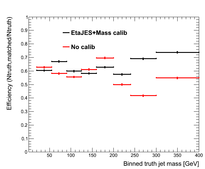
The efficiency (Is the reco jet matched to this truth jet in the same bin as this truth jet?) and the purity (Is the truth jet matched to this reco jet in the same bin as this reco jet?) are shown for CamKt12LCTopo jets before and after the D.M. calibration. Miguel Villiplana has also done this for AntiKt10 jets and sees very similar results.
Jet cleaning Cambridge Aachen (R=1.2) versus AntiKt (R=0.6)
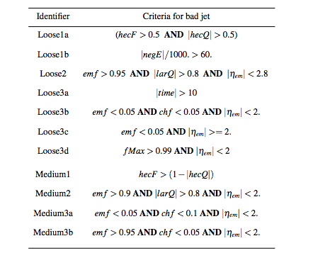
The recommended cleaning cuts for release 16 analyses are shown in this table:
and a comparison between the distributions of each of these variables for AntiKt6 and CamKt12 LCTopoJets is below. The green lines indicate the location of cuts (although these are combined, not taken singly, as can be seen in the table above.) and the arrows indicate the area of each plots that we are interested in looking at.
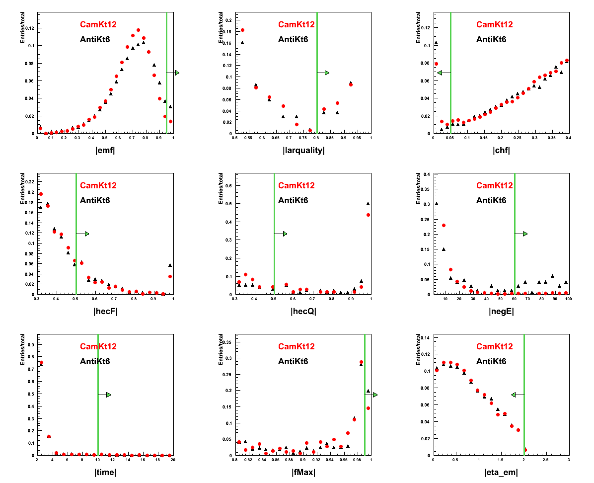
— Sergei Chekanov 2011/03/16 17:57