Jas4PP program is a data-analysis environment for detector and physics studies of future circular colliders. Jas4PP is a merge of several open-source Java projects, such as

• lcsim.org developed at SLAC
• Many file formats used in HEP, including ROOT5 / 6(partially). See Section supported file formats.
• GROOT and XROOTD - data visualization and I/O used at JLab
• j4np-physics - Physics vectors from JLab
• FreeHep developed at SLAC
• DataMelt (community edition) from jWork.ORG
• hs-tools of HepSim developed at ANL.
• Additional libraries such as Apache Common Nath3, JFreeChart and other.
• Various physics packages for statistics, limits settings etc.

The program is designed to work using the following languages:

• Java (+8 version)
• Python language using Jython 2.7.2 (which is compatible with the 2.7.2 version of CPython)
• Groovy (version 3.0.6) https://groovy-lang.org/

The installation does not have external dependencies. To run Jas4pp, you need to install Java. To check you Java installation, run “java -version”. One can find Oracle JDK or JRE versions from the Oracle download link. OpenJDK can be downloaded from https://openjdk.java.net/.

You can download the Jas4pp program using the download page. Then run these commands to install the package using Linux/Mac with the “bash” shell:

bash> wget https://atlaswww.hep.anl.gov/asc/jas4pp/download/current.php -O jas4pp.tgz
bash> tar -zvxf jas4pp.tgz
bash> cd jas4pp
bash> source ./setup.sh # takes 5 sec for first-time optimization
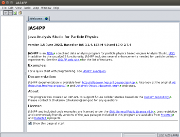
bash> jaspp   

The last command starts Jas4PP GUI:

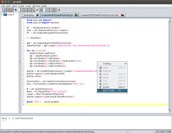
Use this GUI to explore examples with data visualisation shown in the main window: [JAS4PP examples]-[Python examples] and then [F2] (or use the mouse menu) to execute:

If you run Jython/Groovy code in a batch mode, use the following commands:

bash> fpad code.py     # execution of Python/Jython code
bash> fpad code.groovy # execution of Groovy code  

You are ready to run over any file with truth-level (ProMC or LCIO files) and detector-simulation information (LCIO files) from HepSim repository. Here is a list of Jas4pp commands:

jaspp          # start Jas4pp with preconfigured HEP plugins (Linux/Mac with bash)
jaspp.bat      # same for Windows
fpad           # run Jython scripts in a batch mode (Linux/Mac with bash) 
fpad_edit      # start a minimalistic Python editor "FPAD") and Jython shell
fpad_edit.bat  # same for Windows
gconverter     # geometry converters
gconverter_gui # same in GUI mode
hs-help        # shows commands to access data from the HepSim repository

Use these programs for:

• Downloading and searching HepSim data
• Processing ProMC files from HepSim
• Running over SLCIO files with Geant4 simulated / reconstructed events.
• Data analysis (jets, physics vectors, histogram packages, limit settings, etc.)
• Visualization of reconstructed events using Wired4 display

You can find more details in HepSim web page.

We recommend to use Groovy for analysis programs. One advantage of Groovy is that the code execution for large loops is a factor 12 faster than for Jython and CPython). See the benchmark. All HEP Jas plugins are included (and some of them were modified to work with DataMelt).

Jas4pp can be extended by putting external jar files in the directory “lib/user”, or linking pure-Python modules.

All examples of Jas4pp are collected in the directory “examples”. Run them as:

fpad examples/dmelt/histo1.py                 # DMelt histogram example
fpad examples/groot/histogram1d.py            # GROOT histogram example
fpad examples/jaida/Fit.py                    # Jas/Aida fit example
fpad examples/hepsim/pythia6_zpole_tautau.py  # run over HepSim Monte Carlo data

The last example from the HepSim web page prints the pT distribution of e, mu, taus. You can also run these examples as “fpad_edit file.py” or using the Jas-like environment (i.e. jaspp program).

You can find many examples from HepSim validation page (ProMC) and LCIO validation page.

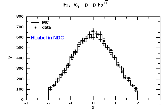
Here is an example of how to compare data points with a histogram using DMelt classes. Run this script as “fpad file.py”, or open it in the Jas4pp editor and run this script.

from java.awt import *
from java.util import Random
from jhplot  import *
 
c1 = HPlot()
# c1.doc()  # view documentation
c1.setGTitle("F_{2},  x_{γ}  #bar{p}p F_{2}^{c#bar{c}}") 
c1.visible(1)
c1.setAutoRange()
c1.setMarginLeft(85) # make space for Y label
c1.setNameX("X")
c1.setNameY("Y")
 
h1 = H1D("MC",25, -2, 2.0)
h1.setPenWidthErr(2) # line width
h2 = H1D("data",25, -2, 2.0)
 
r=Random()
for i in range(10000):
   h1.fill(r.nextGaussian())      
   h2.fill(r.nextGaussian())          
 
p1=P1D(h2) # convert to X-Y array 
c1.draw(h1)
c1.draw(p1)
# c1.drawStatBox(h1)
 
# set HLabel in the normilised coordinate system
lab=HLabel("HLabel in NDC", 0.18, 0.7, "NDC")
lab.setColor(Color.blue)
c1.add(lab)
 
c1.update()
c1.export("image.eps") 

Run this example in Jas4pp and look at this image:

Jas4pp supports the following file formats:

• ROOT6 (read only). Also ROOT versions 3,4,5 are supported for limited number of ROOT objects. XROOTD is included
• LCIO (read/write)
• ProMC (read/write)
• ProOI (read)
• HiPO file format (read/write)
• HepRep (read)
• AIDA XML-format, including compression (read/write)
• STDHEP
• All I/O file formats supported by Python 2.7 (or pure-Python external modules)
• All I/O file-format methods from Java

These file formats are natively supported in Jython/Python, Groovy and Java codes.

Jas4pp natively reads commonly used objects and data structures from ROOT files (versions 3, 4, 5 and 6). ROOT files can be opened using the Jas4pp menu [File]-[Open data source]-[Root file] (*.root).

In addition, one can work with ROOT files using Jython/Python and Groovy scripts. One can find some examples in the directory “examples/root”. Here is a Jython/Python example showing how to read a simple ROOT tree:

from  hep.io.root.interfaces import TTree
from  hep.io.root import RootFileReader
 
reader = RootFileReader("ntuple_tree.root")
 
tree = reader.get("tree");
maxevents=tree.getEntries()
 
leaves = tree.getLeaves()
nrleaves=leaves.size()
 
print "Nr of events=",maxevents
print "Nr of leaves=",nrleaves
 
print "Leaves:"
for l in xrange( nrleaves ):
   print "Leaf=",(leaves.get(l)).getName()
 
print "Run over events"
f0=leaves.get(0);
f1=leaves.get(1);
f2=leaves.get(2);
for i in xrange(tree.getEntries()):
      print f0.getValue(i), f1.getValue(i), f2.getValue(i)

The example directory also shows how to read histograms. Similar examples can be made using Java or Groovy scripting.

The supported ROOT interfaces are:

There are other interfaces for reading complex root trees as those from Delphes fast simulations.

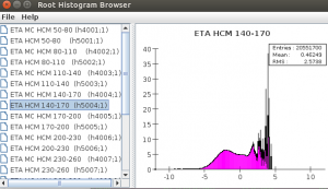
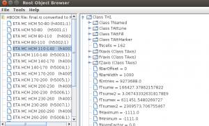
One can browser ROOT histograms (or other objects) using this:

import rootio
rootio.HBrowser("histograms_root5.root") # browser and plot ROOT histograms 
rootio.Browser("histograms_root5.root")  # browser for ROOT objects

You will see the browsers:

The last image shows the complete class structure of the ROOT file. Thses scripts can be put into Jython or Groovy files and executed as binary programs.

If the ROOT file has custom C++ classes, you need to create Java interface classes and compile them to the jar file and move this jar fil to “lib/user” directory of Jas4pp. To create interface classes for a ROOT file “test.root”, use:

import rootio
rootio.Builder("test.root", None) # create interface classes in the current directory 

This functionality is unchanged compared to FreeHep RootIO library.

Jas4pp can be used for analysis of complex ROOT trees from fast simulations created by the Delphes framework. Many Delphes Monte Carlo files can be found in the HepSim repository. Download an example ROOT file with ttbar+jet events created with Madgraph5 from HepSim:

wget https://mc.hep.anl.gov/asc/hepsim/events/pp/13tev/mg5_ttbar_Njet/rfast102/mg5_ttbar_Njet_001.root

To study the structure of this ROOT file, run the browser:

import rootio
rootio.Browser("mg5_ttbar_Njet_001.root") 

The browser tells how the data are organized inside the ROOT file.

The process the tree “Delphes” from this file, one can write a small code in Python (writing in Groovy and Java is also trivial). Here is a simple code to show a histogram with particle ID:

from  hep.io.root import RootFileReader
 
xf="mg5_ttbar_Njet_001.root" # input file
 
# examine file before doing anything
# import rootio
# rootio.Browser(xf)
 
reader = RootFileReader(xf)
tree = reader.get("Delphes")
branches=tree.getBranches()
print "Nr of events=",tree.getEntries()
print "Nr of branches=",branches.size()
 
for l in xrange(branches.size()):
   print "Branch=",l," name=",(branches.get(l)).getName()
 
particles=tree.getBranch("Particle") # get Particle branch
print "Type:", type(particles)
branches=particles.getBranches();
print type(branches)
for l in  branches:
   print "particle ",type(l), " name=",l.getName()
 
PID=particles.getBranchForName("PID")
leaves=PID.getLeaves();
print PID.getName(), "has", leaves.size();
 
from jhplot import *
h1 = H1D("particle ID",100, -10, 10) # fill a histogram
 
pid=leaves.get(0) # get values with PID for all events
for i in xrange(tree.getEntries()):
      h1.fill(pid.getValue(i))
 
c=HPlot("particle ID")
c.visible()
c.setAutoRange()
c.draw(h1)        

Note this code only works for integer values since we did not specify which value needs to be extracted.

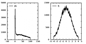
If you need to extract double, float or boolean values, use the Delphes class and its “get” methods, getFloat, getDouble, getInt, and getBool. Here is an example that uses high-level classes to read transverse momentum (PT) and pseudorapidity (ETA) of Monte Carlo particles:

from  hep.io.root import RootFileReader
from rootio import *
 
reader = RootFileReader("mg5_ttbar_Njet_001.root" )
tree = reader.get("Delphes")
branches=tree.getBranches()
print "Nr of events=",tree.getEntries()
print "Nr of branches=",branches.size()
print "Branches:"
for l in xrange( branches.size() ):
   print "Branch=",l," name=",(branches.get(l)).getName()
 
particles=tree.getBranch("Particle")        # generator particles
ptEvents=Delphes.getFloat(particles,"PT")   # get PT array
etaEvents=Delphes.getFloat(particles,"Eta") # get ETA array
 
from jhplot import *
h1 = H1D("PT of particles",100, 0, 100)
h2 = H1D("Eta of particles",100, -4, 4)
for i in xrange(tree.getEntries()):
       pt,eta=ptEvents[i],etaEvents[i]
       for j in xrange(len(pt)):
           h1.fill(pt[j])
           h2.fill(eta[j])
c=HPlot("pT",600,300,2,1)
c.visible()
c.setAutoRange()
c.draw(h1)
 
c.cd(2,1)
c.setAutoRange()
c.draw(h2)

Jas4pp can visualize histograms created by Fortran or C++ code (but without using ROOT). For this, use a light stand-alone library called CFBook (See CFBook). You can compile it using gcc (for C++ programs) or gfortran (for Fortran program). This library creates XML file with 1D and 2D histograms, that can be read by Jas4pp. Here is an example of reading 1D histogram from fortran.xml file:

from jhplot  import *
from jhplot.io import *
 
hb = CFBook()
hb.read("fortran.xml")
print hb.listAll()
print hb.getKeysH1D() # list keys
h1=hb.getH1D(1)        # use the key 1 to retrive H1D
c1=HPlot("Test")
c1.setGTitle("Histograms from a file");
c1.visible(1)
c1.setAutoRange()
c1.draw(h1)

Jas4pp can be used to process LCIO files. It can read and write LCIO files. The examples are given in the directory “example”.

# Example of processing SLCIO files using Jas4pp
# Setup Jas4pp using "source setup.sh".
# Then create the directory "data"  and fill it with SLCIO files using has-get command,
# and run this script as "fpad example.py data"
 
from org.lcsim.lcio import LCIOReader
from hep.io.sio import SIOReader
from hep.lcio.implementation.sio import SIOLCReader
from hep.lcio.implementation.io import LCFactory
from hep.lcio.event import * 
from hep.lcio.io import *
from jhplot import *
from hephysics.particle import LParticle
import math
import os,sys
from java.lang import System;
 
# get directory name from the argument
filename = sys.argv[1]
 
# make list of files..
import glob
files = glob.glob(filename+"/*.slcio")
factory = LCFactory.getInstance()
 
nEvent=0
for f in files:
    print "Open file=",f
    reader = factory.createLCReader()
    reader.open(f) 
    while(1):
        evt=reader.readNextEvent()
        if (evt == None): break
        nEvent=nEvent+1
        # print " file event: ",evt.getEventNumber(), " run=",evt.getRunNumber()
        if (nEvent%100==0): print "# Event: ",nEvent
        col    = evt.getCollection("MCParticle")
        colPF  = evt.getCollection("PandoraPFOCollection");
        colCl  = evt.getCollection("ReconClusters");
        colTr  = evt.getCollection("Tracks");
        colECB = evt.getCollection("EM_BARREL");
        colHCB = evt.getCollection("HAD_BARREL");
 
        nMc=col.getNumberOfElements();
        nPF=colPF.getNumberOfElements();
        nCl=colCl.getNumberOfElements();
        nTr=colTr.getNumberOfElements();
        nECB=colECB.getNumberOfElements();
        nHCB=colHCB.getNumberOfElements();
        # now you can access all data here
 
        # manage memory if too much data 
        del col
        del colPF
        del colCl
        del colTr
        del colECB
        del colHCB
        del evt
 
    reader.close() # close the file
    del reader
    System.gc()    #  force memory cleanup, if needed 

To process SLCIO files from a directory “data”, call this script “example.py as:

fpad example.py data

The script open each file, and access every container in the file. Note that we explicitly mange memory in case of very large files, forcing the garbage collector for each file. In many cases, this is not needed since JVM takes care of memory problems.

See LCIO validation page for more examples.

Jas4pp natively reads miniDST files created for the ILC studies. Here is the example showing how to make a Z-boson peak from a miniDST file. This file is described in this recent tutorial [https://indico.fnal.gov/event/45031/overview].

Here is the example:

wget https://atlaswww.hep.anl.gov/asc/jas4pp/data/rv01-16-p10_250.sv01-14-01-p00.mILD_o1_v05.E250-TDR_ws.I106479.Pe2e2h.eL.pR-00001-ILDminiDST.slcio

The run this code that reads this files and creates the Z-boson mass. The code is shown here:

from hep.lcio.implementation.io import LCFactory
from hephysics.particle import LParticle
from jhplot import  HPlot,H1D
from math import sqrt
import glob
 
files=["rv01-16-p10_250.sv01-14-01-p00.mILD_o1_v05.E250-TDR_ws.I106479.Pe2e2h.eL.pR-00001-ILDminiDST.slcio"] 
factory = LCFactory.getInstance()
 
h1= H1D("Mass",50,0,200)   # create a histogram
h1.setFill(True)
nEvent=0
for f in files:
  print "Open file=",f
  reader = factory.createLCReader()
  reader.open(f)
  while(1):
     evt=reader.readNextEvent()
     if (evt == None): break
     nEvent=nEvent+1
     # print " file event: ",evt.getEventNumber(), " run=",evt.getRunNumber()
     if (nEvent%100==0): print "# Event: ",nEvent
     strVec = evt.getCollectionNames()
     if nEvent == 1:
            for col in  strVec:
                           print col
     col = evt.getCollection("IsolatedMuons")
     muons=[]
     for i in range( col.getNumberOfElements() ):
          track=col.getElementAt(i)
          mom=track.getMomentum() 
          px,py,pz=mom[0],mom[1],mom[2] 
          ee=sqrt(px*px+py*py+pz*pz)
          muons.append( LParticle("muon",px,py,pz,ee,0.105) )
     col = evt.getCollection("Refined2Jets")
     jets=[]
     for i in range(col.getNumberOfElements()):
          jet=col.getElementAt(i)
          mom=jet.getMomentum()
          px,py,pz=mom[0],mom[1],mom[2]
          ee=sqrt(px*px+py*py+pz*pz)
          p=LParticle("jet",px,py,pz,ee,0)
          jets.append(p)
 
     if (len(muons)==2): # mass
           obj=muons[0]
           obj.add(muons[1])
           mass=obj.calcMass()
           h1.fill(mass)
           #print(mass)
 
     del col,evt
  reader.close() # close the file
  del reader
 
c1 = HPlot("=HepSim=",600,400) # plot histogram
c1.setNameX("Mass")
c1.setNameY("Events")
c1.setSubTicNumber(0,5)
c1.visible(True)
c1.setAutoRange()
c1.setRangeX(0,200)
c1.setRangeY(0,10000)
c1.setMarginLeft(90)
c1.draw(h1)

Jas4pp can be used to write Jython scripts to validate HepSim ProMC files. Please look at HepSim manual. All such java classes can be accessed using Java, JShell, Groovy and Jython programs.

One can learn about Jas4pp classes using Jas4pp API documentation. These classes can be used in Java, JShell, Groovy and Jython analysis programs.

Jas4pp uses histogram packages supported by both DMelt (community edition), JAIDA (FreeHep) or GROOT (JLab). DMelt provides programming API similar to PyROOT and with classes named conveniently to reduce code verbosity.

Here are a few most common classes:

• HPlot - canvas to show X-Y data and histograms in 2D
• HPlot3D - canvas to show X-Y-Z data and histograms in 3D
• H1D - 1D histogram
• H2D - 2D histogram
• P1D - X-Y container with support of 2-level errors
• j4np-physics - Physics vectors

The main canvas to show histograms H1D and data points P1D is HPlot. To process scripts in a background without a pop-up HPlot, use method “visible(False)”, and set sys.exit(0) at the end of the scripts. You can also use the JAIDA to make histograms (Histogram1D or Histogram2D). In addition, data are saved in the form of XML (with the extension ”.jdat“) files. Look the manual http://handwiki.org/wiki/DMelt:Start.

• PromcUtil convenient method to fill arrays with particles from ProMC files
• LParticle a HEP particle with the Lorentz transformations
• FastParticle a HEP particles with precomputed Et2,Eta,Phi for jet algorithms.
• Physics vectors typical HEP physics vectors the Lorentz transformations
• JetN2 recommended kt-type jet clustering algorithms (kT, anti-kT, CA) implemented in Java using N^2 approach, similar to the FastJet algorithm. Recommended for hadron collisions
• SCJet traditional kt-type jet clustering algorithms (kT, anti-kT) for pp implemented in Java using N^3 approach (slow)
• Jets and event shapes traditional jet algorithms and event shapes for e+e- from FreeHep (Geneva, Jade, Durham jets)

Java implementation of the longitudinally invariant kT and anti-kT clustering algorithms uses the E-scheme to combine particles (p1+p2) and Eta-Phi space (not Rapidity-Phi). Also, Cambridge/Aachen jets are supported. HepJet on github shows benchmarks of the Java implementation of the anti-KT with the original FastJet package.

You can build the standard kt-jets using PromcUtil, followed by the KTjet class.

GROOT is a light-weight package for Java visualization created at JLAB. The full API of GROOT can be found in GROOT API page. There is also GROOT Wiki describing some features of GROOT.

Please look at the examples inside the directory “examples/groot”.

You can run Jas+Wired to visualize the simulated events. The Wired program is included in Jas4pp, so you simply run it as:

./jaspp

This will start a Jas3-like environment with all needed plugins. Then copy the detector geometry file from the detector repository.

wget http://atlaswww.hep.anl.gov/hepsim/soft/detectors/sidloi3.tgz -O - | tar -xz;

This will create a directory “sidloi3”. This detector corresponds to “rfull001” tag used for the reconstruction of pythia6_zpole_ee (Z→e+e-).

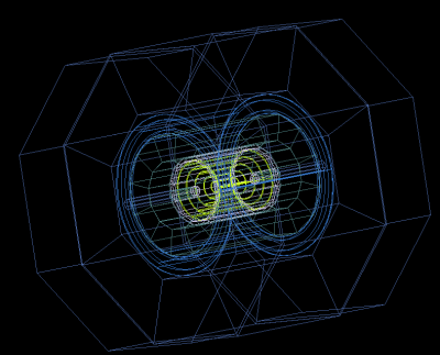
Now we can visualize the detector as [File]-[Open data source]-[HepRep] XML and select the file “sidloi3.heprep” from sidloi3.tgz: This is how to do this using the command line:

./jaspp  sidloi3.heprep

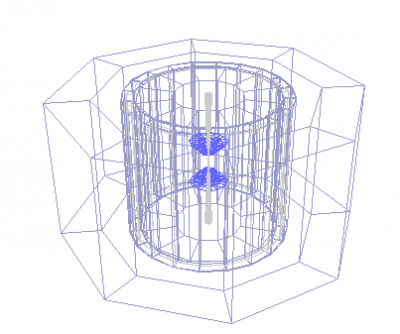
You will see the detector layout:

Now, we will read the event: Open any *.slcio file you copied from HepSim as [File]-[Open data source]-[LCIO] file. Then click a small button [Go] (top menu bar). It will process events. Then select again [File]-[New]-[Wired 4 view]. You will get an image in the Wired4 display. Now press [Go] again to look at next event.

If you want to see how data records are organized inside the slcio file, do this [File]-[New]-[LCSim Event browser]

Here is an example of how to visualize LCIO files from the HepSim repository

wget http://mc.hep.anl.gov/asc/hepsim/events/misc/pgun/pgun_eta35_muon//rfull009/pgun_muon1024gev_001_pandora.slcio
./jaspp pgun_muon1024gev_001_pandora.slcio

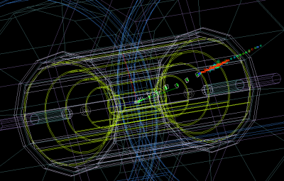
Click “Go” in the menu. Now you can open the event browser or Wired event display. Look at event record as “File→New→Event Browser”. Similarly, visualize the event as ” File→New→Wired4 View“. It shows an black window on the left. Then go to the next event, click “Go next” in the menu. This image illustrates a single electron event:

Similarly, you can view any events form the HepSim directory.

Generally, when you open a SLCIO file from the HepSim, you do not need to load the geometry file. The geometry file will be downloaded automatically from HepSim and will be put to ”.lcsim/cache/“ inside your home directory. Then go to the next event, click “Go next” in the menu. This image illustrates a single electron event:

Similarly, you can view any events form the HepSim directory.

Generally, when you open a SLCIO file from the HepSim, you do not need to load the geometry file. The geometry file will be downloaded automatically from HepSim and will be put to

.lcsim/cache

(inside your home directory).

Visualization of complex 100 TeV events are shown in the HepSim manual.

(contribution from N.Nikiforou):

You can also visualize the detector using ROOT. Here are a few steps: Locate the file detector.gdml inside the file detector.zip (where “detector” shows the name of the detector).

slic -g detector.lcdd -G detector.gdml

Once you have the GDML file, you can use ROOT to visualize it. You just need to make sure the ROOT installation has openGL/GDML support (CERN AFS installations have it for sure). At the ROOT prompt do:

TGeoManager::Import("detector.gdml");
gGeoManager->GetTopVolume()->Draw("ogl");

This should popup an OpenGL display with the detector which you can clip, pan, rotate etc. You will the image as shown here:

HepSim wiki explains how to use Jas4pp for physics and performance studies of future colliders. For example, this page shows how to visualize complex 100 TeV events. Such complex events were featured by this general article. Jas4pp is currently used for FCC, CEPC and EIC studies.

• S.Chekanov (ANL, main developer)
• E.May (ANL, debugging, Wired4)
• D.Blyth (speedup rendering of events and ProIO support)
• N.Nikiforou
• G.Gavalian (JLab)
• Khushi Taori (ANL SULI 2021 student). ROOT6 support validation

• http://jas.freehep.org/jas3/ - JAS3
• http://java.freehep.org/ - FreeHep
• https://datamelt.org - DataMelt
• https://confluence.slac.stanford.edu/display/ilc/ILC+Detector+Simulation+FAQ - SLIC
• https://confluence.slac.stanford.edu/display/ilc/LCSim+Tutorials - SLIC
• https://atlaswww.hep.anl.gov/asc/promc/ ProMC file format
• http://lcio.desy.de/ LCIO file format

Jas4pp is licensed under GPL. The source code available on Github (under construction).

— Sergei Chekanov 2016/03/23 21:53